Testing the clock model in BactDating

Initialisation

library(BactDating)
library(ape)
set.seed(0)

Data generated from strict clock model

We start by generating a coalescent tree with 10 leaves sampled at regular intervals between 1990 and 2010, and a coalescent time unit of 5 years:

dates=1990:2010
phy=simcoaltree(dates,alpha=5)
plot(phy,show.tip.label = F)
axisPhylo(backward = F)

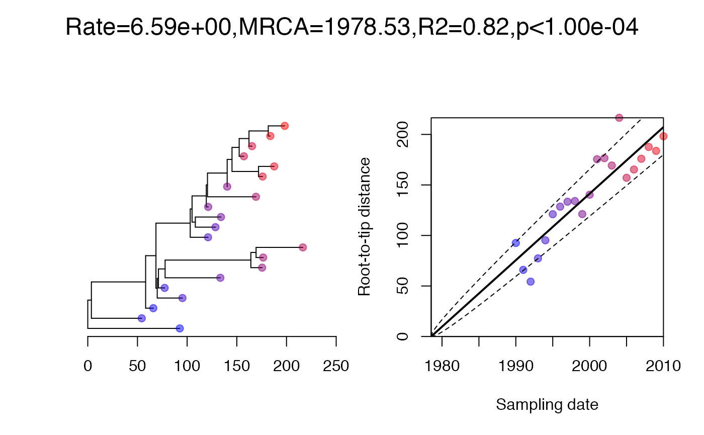
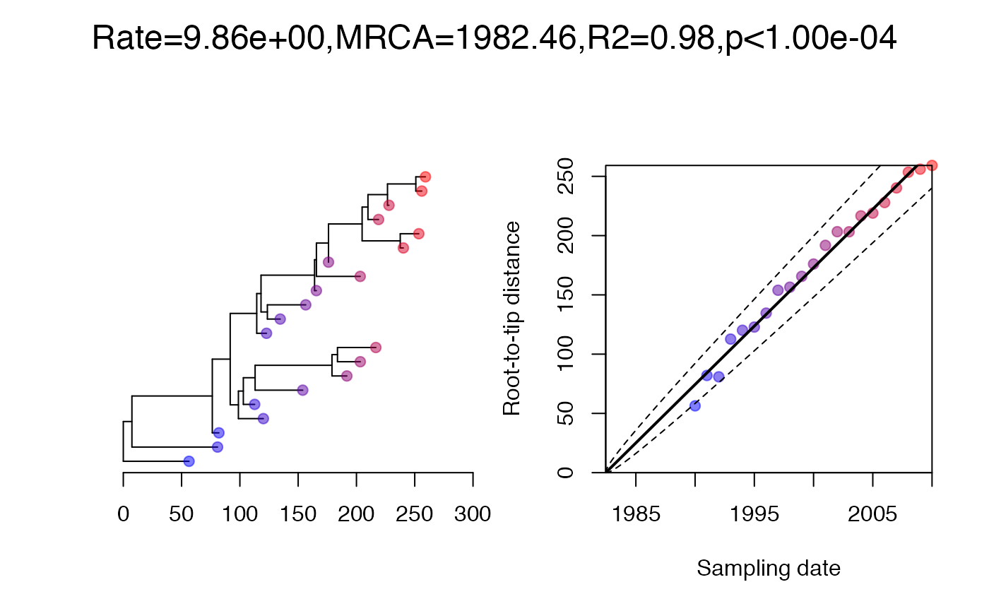
On each branch we observe a number of substitutions which is distributed \(\mathrm{Gamma}(rl,1)\) where \(l\) is the branch length and \(r=10\) per year is the substitution rate. We can simulate an observed phylogenetic tree and perform a root-to-tip analysis as follows:

obsphy=simobsphy(phy,mu=10,model='strictgamma')
res=roottotip(obsphy,dates)

Analysis of data from strict clock model

We run the dating analysis as follows:

res=bactdate(obsphy,dates,updateRoot=F,model='mixedgamma')
plot(res,'trace')

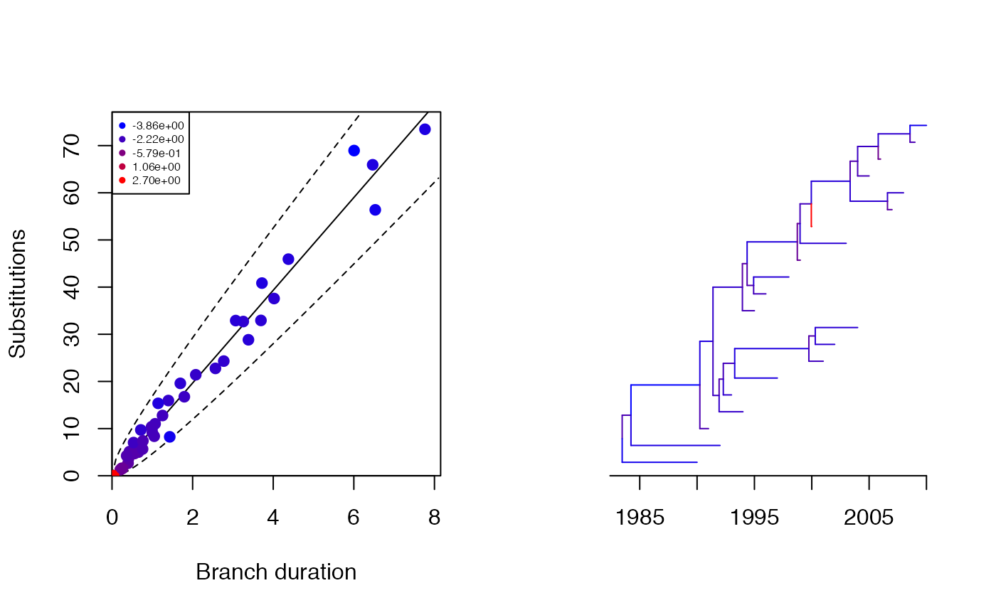
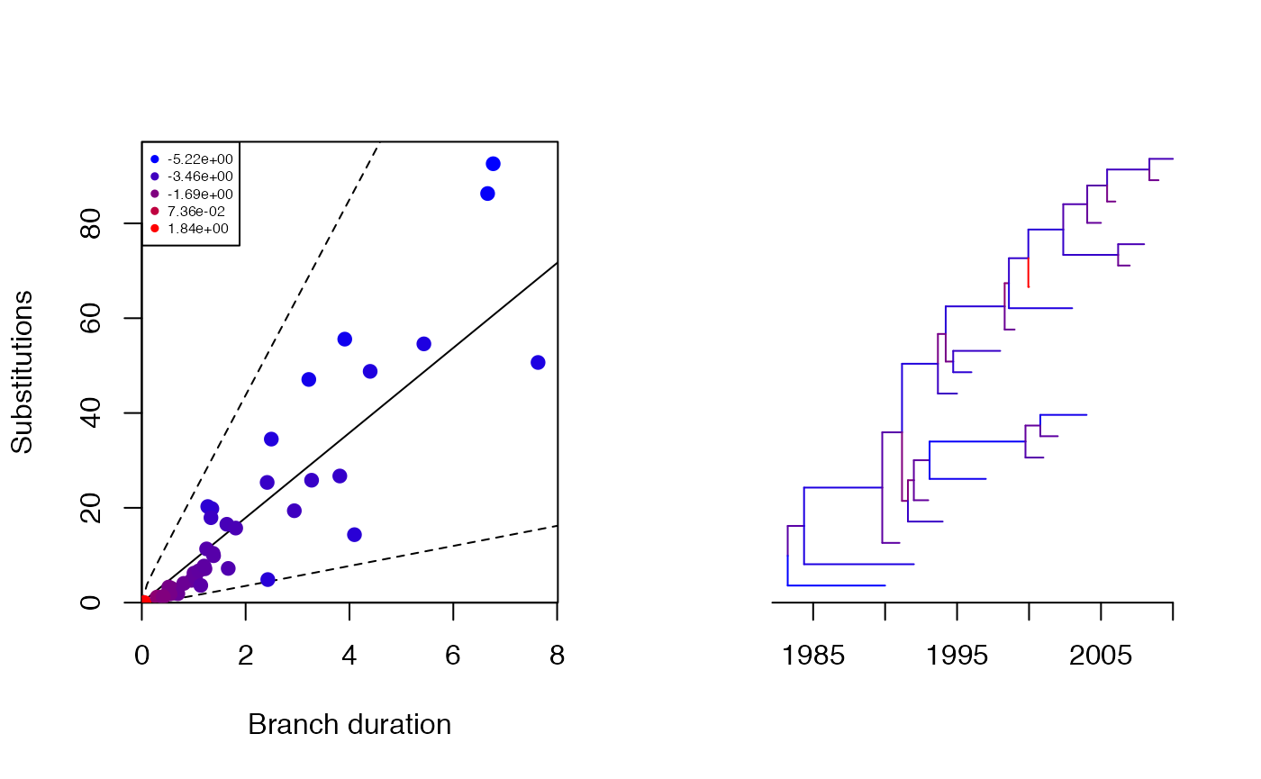
print(res$pstrict)

## [1] 0.986

Let’s see how each branch contributes to the overall likelihood:

plot(res,'scatter')

Data generated from relaxed clock model

Let’s start again with a new dataset generated using the relaxed clock model:

set.seed(0)
obsphy=simobsphy(phy,mu=10,model='relaxedgamma',sigma = 5)
res=roottotip(obsphy,dates)

Analysis of data from relaxed clock model

We run the analysis as previously:

res=bactdate(obsphy,dates,updateRoot=F,model='mixedgamma')
plot(res,'trace')

print(res$pstrict)

## [1] 0