Demonstration of DetectImports principle

Xavier Didelot

2025-11-19

Initialisation

library(DetectImports)
library(ape)
set.seed(0)

Simulation with constant population size

For initial simplicity, consider that the local population has constant effective population size $N_e$.

Ne=function(t){return(5)}
tree=simCoal(seq(2000,2020,0.05),Ne)
plotBoth(tree,Ne)

Coalescent intervals

We consider the leaves $k=1..n$ in increasing order of date. Let $s_k$ denote the date of leaf $k$, we have $i<j \implies s_i<s_j$. The $k$-th leaf has to coalesce with the genealogy formed by the $(k-1)$ first leaves. Let $C_k$ denote the sum of branch lengths in the genealogy formed so far between the time of leaf $k$ and the time where it coalesces with an ancestor of a previously considered leaf. We call $A_i$ the ``coalescent interval’’. Let’s plot $C_k$ on the y-axis against $s_k$ on the x-axis:

plotCoalInt(tree)

Detection of imports

Imports are likely to have $C_k$ greater than expected if transmission happened only locally. In the case where the location population size is constant equal to $N_e$, $C_k$ is exponentially distributed with mean $N_e$. So we can detect imports by looking for coalescent intervals that are greater than this. Since $N_e$ is unknown, we need to estimate it from the data. A simple estimator would be to take the mean of the $C_k$, but since we suspect that some $C_k$ are affected by imports, it is preferable to use an estimator based on the median: $$\hat N_e=\frac{\mathrm{median}(C_{1..n})}{\mathrm{ln}(2)}$$ Of course here there are no imports:

res=detectImportsFAST(tree,constant=T)
plot(res,'scatter')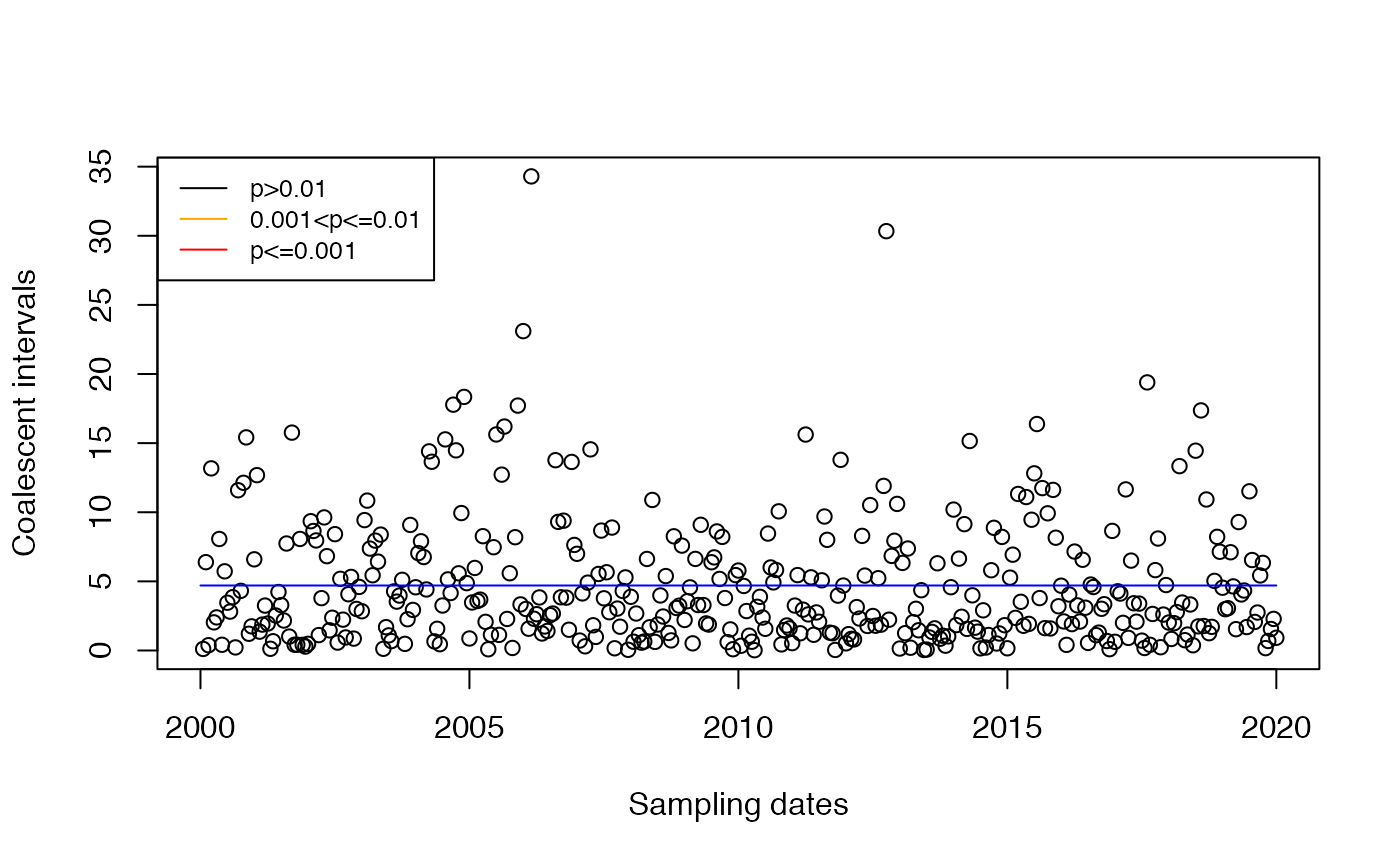

Simulation with varying population size

Now we consider that the effective population size is not constant but is a continuous function $N_e(t)$ of time.

set.seed(0)
Ne=function(t){if (t>2010|t<2005) return(2) else return(10)}
tree=simCoal(seq(2000,2020,0.05),Ne)
plotBoth(tree,Ne)

Coalescent intervals

The coalescent intervals $C_k$ are no longer exponential and no longer iid as in the case of a constant population size. But we can still compute them and plot them as before:

plotCoalInt(tree)

Bad test

If we apply the same test as before, we will get some false positives in the detection of imports:

res=detectImportsFAST(tree,constant=T)
plot(res,'scatter')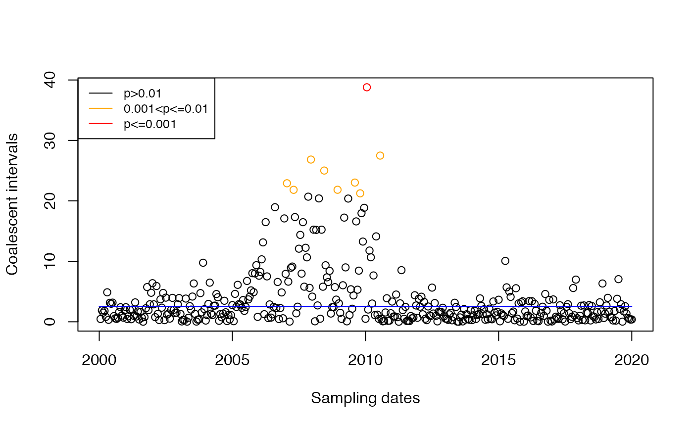

Detection of imports

Outliers in the distribution of $C_k$ against $s_k$ are likely imports. The distribution $p(C_k|s_k)$ is unknown and complex in the general case. We use a test in which the distribution is assumed exponential with time-changing mean $\hat N_e(t)$ estimated. This is not quite correct since the distribution is not exponential, but matching the mean is a good first step. As a first attempt, let’s consider the estimator based on the median of other coalescent intervals around the same time: $$\hat N_e(s_k)=\frac{\mathrm{median}(C_{j\neq k\mathrm{~with~}|s_k-s_j|<\epsilon})}{\mathrm{ln}(2)}$$

This estimator is used in the fast test of DetectImports:

res=detectImportsFAST(tree,constant=F,epsilon=1)
plot(res,'scatter')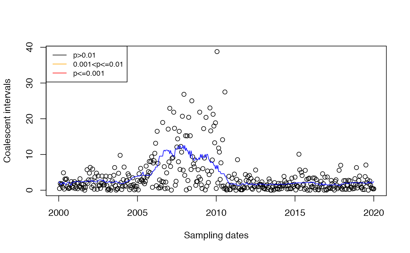

We can see that the false positives are no longer present. In the DetectImports paper, we develop a test based on the same principle but using Bayesian statistics.